1. Introduction: If We Can "Forward-Simulate"  a Spectrum, We Must Be Able to "Inverse-Solve" a Structure

Before discussing the inversion capability of the True FP algorithm, we start with a fundamental but often overlooked fact:

If the structure, composition, number of layers, and thickness of a sample are given, the True FP algorithm can precisely simulate its theoretical XRF spectrum on any instrument—purely from physics.

In other words:

Known structure → FP algorithm → Spectrum

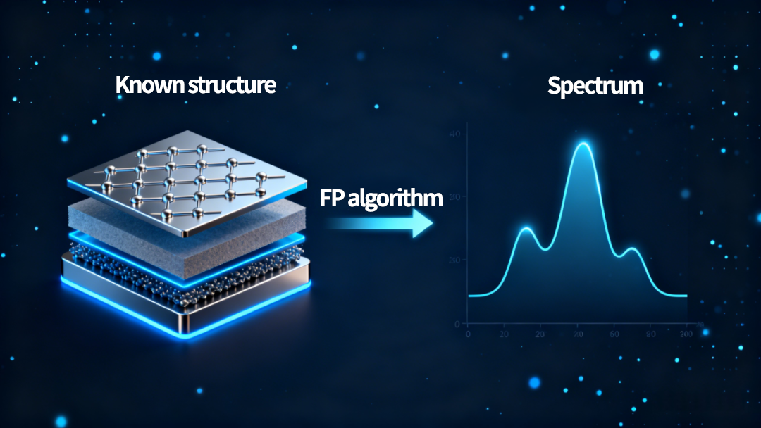
This is a deterministic forward modeling process based entirely on physics.

If FP can compute a spectrum from a structure, then the reverse must also hold:

Structure → Spectrum 

implies 

Spectrum → Structure.

This is the physical foundation of inversion.

Inversion is not a heuristic technique —

it is the inevitable consequence of possessing a complete forward physical model：

  ·  The more complete the forward model is,

  ·  the more feasible inversion becomes,

  ·  and the more accurate the inversion will be.

Therefore:

The True FP algorithm does not "fit curves" ; it performs physical reasoning over the entire spectrum.

Only an algorithm that possesses a complete forward process can truly solve the inverse problem.

2. Forward vs Inverse Problems: Two Completely Different Ways of Understanding XRF

✔ Forward Problem

Structure known → Compute spectrum

Example:

"If sample like this, what should its spectrum look like?"

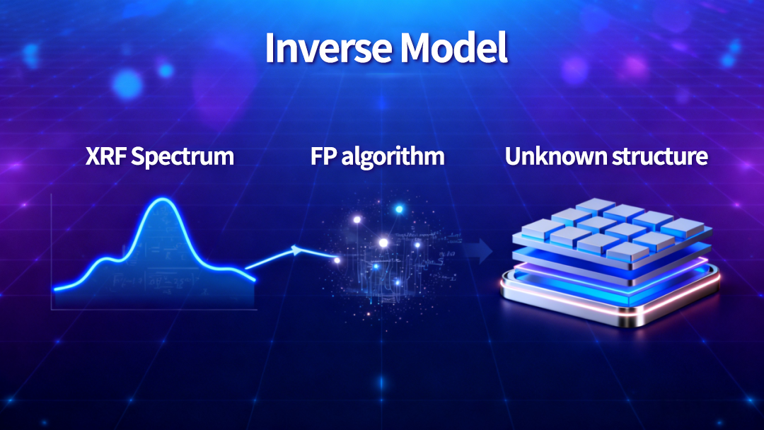
Inverse Problem

Spectrum known → Reconstruct structure

Example:

"With such a spectrum, how many layers exist? What are their compositions and thicknesses?"

Traditional empirical algorithms operate cover only a narrow slice of the forward problem:

they convert peak intensities into concentrations through regression.

They cannot solve the inverse problem.

The True FP algorithm solves the full inverse problem:

Given only a spectrum, it infers the structure, thickness, and elemental distribution across layers.

3. Why Traditional Algorithms Cannot Perform Inversion

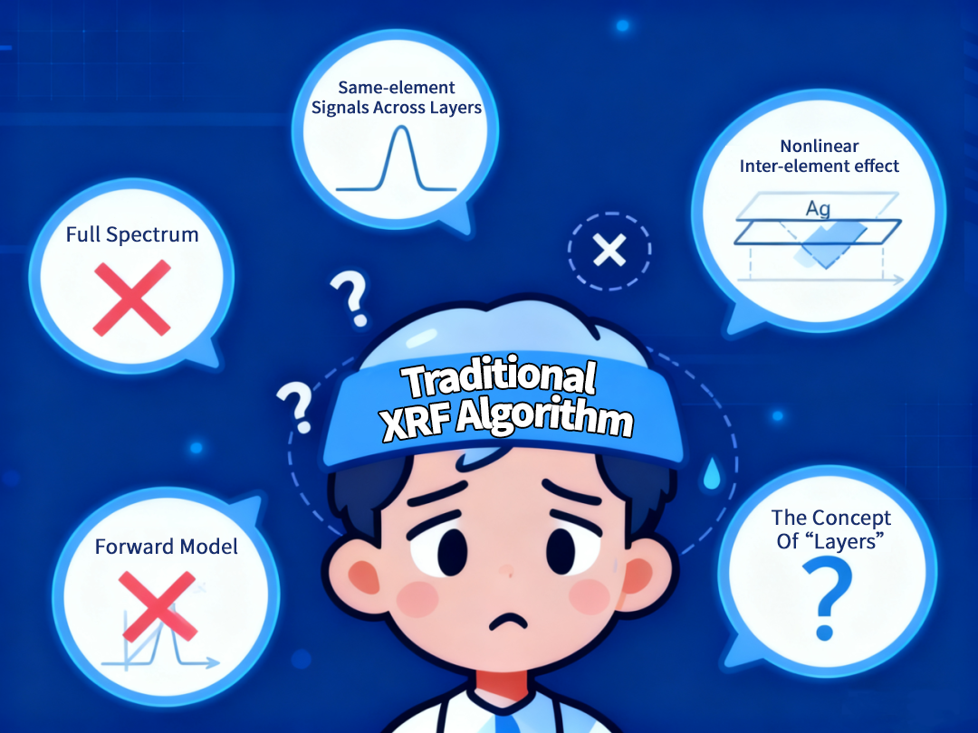
This is not a matter of algorithm design—it is a limitation of principle:

1)They rely solely on peak height—not at the full spectrum

They neglect:

  ·  background curvature

  ·  absorption edges

  ·  peak broadening

  ·  peak shifts

  ·  low-energy attenuation trends

  ·  energy-dependent residuals

2) Nonlinear inter-element effects are not modeled

Au–Cu, Au–Ag–Cu, Ni–P, and most real alloys exhibit strong nonlinear absorption.

3) They cannot separate same-element signals across layers

Ag in surface layer vs Ag in substrate

Cu in alloy vs Cu in base

→ appear identical in empirical algorithms.

4) They cannot express the concept of  "layers"

Their mathematical structure inherently assumes a single averaged material.

5)Most critically: They have no forward model

And without a forward model, inversion is impossible.

Empirical algorithms fit data; the FP algorithm solves the underlying physics.

4. The Core of the True FP Algorithm: Full-Spectrum Inversion & Automatic Modeling

The True FP algorithm is not curve fitting.

It is a physics-driven spectrum reconstruction engine.

The entire inversion process can be summarized as:

Hypothesize → Simulate → Compare → Adjust → Match

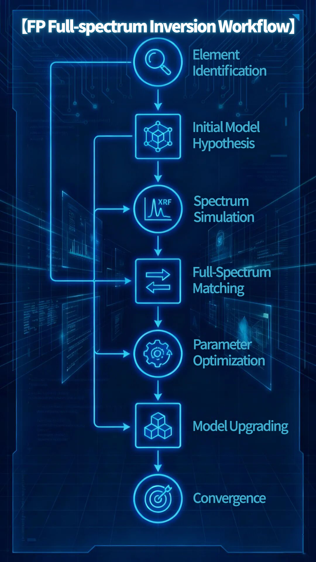
FP full-spectrum inversion workflow

5. Blind Sample Inversion: From "Knowing Nothing"  to "Full Structure Reconstruction"

Input: a single unknown spectrum containing Au, Ag, Cu, Zn, Pd, Sb.

FP inversion proceeds automatically:

 
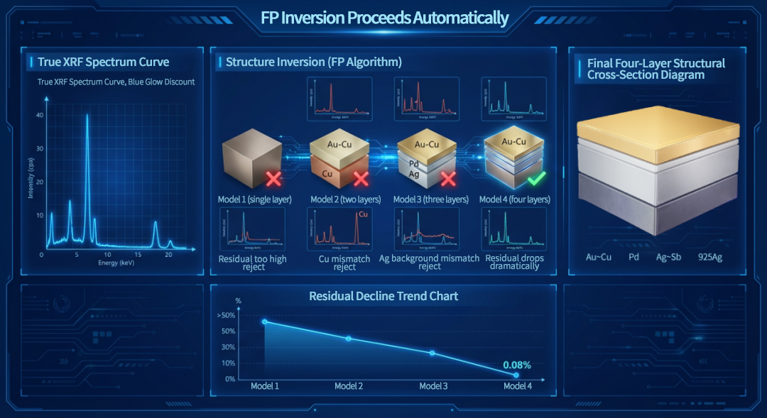
  ·  Model 1 (single layer): residual too high → reject

  ·  Model 2 (two layers): Cu mismatch → reject

  ·  Model 3 (three layers): Ag background mismatch → reject

  ·  Model 4 (four layers): residual drops dramatically

  ·  Further optimization → residual converges to 0.08%

Output structure becomes:

Au–Cu / Pd / Ag–Sb / 925Ag

All without telling the algorithm:

  ·  the number of layers

  ·  the order of layers

  ·  the compositions

  ·  or any prior knowledge

True FP performs autonomous modeling.

It does not  "guess" —it calculates.

6. The Value of the True FP Algorithm: Explainability, Verifiability, Traceability

FP provides three capabilities empirical algorithms never will:

✔ Explainability

Every layer has a clear physical reason:

absorption behavior, edge structure, inter-element excitation, background slope.

✔ Verifiability

Residual plots provide quantitative evidence of correctness.

✔ Traceability

Results can be reconstructed from physics, not from regression coefficients.

The FP algorithm is not a black box.

It is a transparent physical reasoning engine.

7. Conclusion: Turning an XRF Instrument into a Reasoning System

Traditional XRF algorithms measure "peak intensity".

The True FP algorithm interprets the entire spectrum.

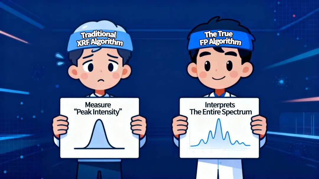
This is a transformation from:

  ·  measurement → inference

  ·  peak fitting → spectrum reconstruction

  ·  empirical → physical

  ·  single-layer → multi-layer

  ·  known samples → blind samples

The essence of the True FP algorithm is this:

It gives XRF the ability to understand materials—not just report numbers.